Closing The Loop

In my last post I showed that there was a lunar seismic event on May 29th, 1972 that seems likely to have been caused by the impact of the Apollo 16 Lunar Module Orion. Knowing the time of this event is an extremely valuable clue to help locate the point of impact. I showed in an earlier post that the impact locations of a randomized set of simulations varied with time, shifting gradually westward on the Moon for later impact times. If we have a target impact time, we can run more trials, and look for impacts at the right time. Then we can check the area where these occur…and hopefully the area is small enough to make a visual search practical. 

There is a problem with this "shotgun" strategy though. If we generate the trials randomly the impact times with be spread out over days. Only a very small fraction of the runs will happen to hit the Moon around the desired time. Even though each simulation completes in just 8 minutes, it would take thousands of trials to build up a good database of timely impacts. We need a better way.

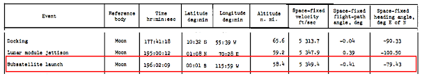
In looking at the data from the first trials, there is a pattern which might offer a way forward. Each simulation starts with six numbers that represent the initial state of Orion’s orbit. The numbers represent the position (latitude, longitude, and altitude) and velocity (speed and direction) of the spacecraft when it was jettisoned. To generate a set of simulations, each of these six parameters is perturbed randomly. The hope is that the random variations will make up for any errors of precision Orion’s initial state. Hopefully all the variation covers the true initial state. In looking over the six input variables, and comparing to the results, an interesting pattern emerges. 

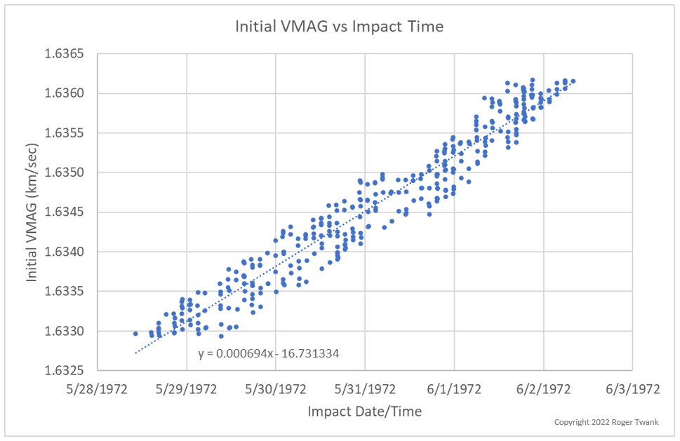
Figure 1: Impact Date versus initial VMAG

Figure 1 is a plot of the speed parameter, VMAG, versus the resulting simulated impact date. Each dot in the figure represents one simulation run.  What is interesting is the trend in the data, as summarized by the dotted trend line. Simulations resulting in an earlier impact had, on average, smaller VMAG values, and those resulting in later impact had larger VMAG values. According to the trend line, on average a change in VMAG of just 0.000694 km/sec resulted in a one-day change in the impact. That’s 69 cm/sec, for a parameter that is in the range of 1.6 km/second. So a very slight nudge, less that 0.05%, leads to in a one-day shift in the impact date.

Therefore, the strategy is to first run a randomized set of simulations. Then calculate the number of days that the resulting impact “missed” the desired target impact time. Multiply this error by 69 cm/second, and add this “nudge” factor to the initial VMAG value, to generate a new VMAG value. Then re-run the simulation with the new VMAG value. By using the outcome to feed back into the initial conditions, we are "closing the loop". Let's give it a try. 

Figure 2: Impacts converging on the desired time after several rounds of VMAG nudging

Figure 2 shows the results using this technique. On the left side, after the initial run, the impact times range from 2 days early to 4 days late compared to the target time. For each case, I calculate the “nudge” value, update VMAG, and run the simulations again. After one round of this nudging, the results are much more concentrated around the target date. Everything is within +/-1 day of the target. Now I can repeat the process a second time, again adjusting the VMAG values by ~69 cm/sec per day of error. Since the errors are fractions of a day, the nudges are proportionally smaller. After two rounds, I have a large set of simulations which are impacting around the desired time. Voila...it’s working well!

Isn’t this cheating? We started by generating random variations, but now we are selectively adjusting one of those values. VMAG is no longer random. That is true, but there is still value in this technique. Take a look at the progression of VMAG values in the trials, shown in Figure 3. (These are sorted from lowest to highest initial values.) The values for VMAG vary randomly with a total of 6 meters/sec variation around the nominal value. (This is a very generous variation, given that NASA said in 1972 that the doppler tracking enabled them to measure the spacecraft speed to within 0.5 feet/sec.) After two rounds of nudging, the variation in VMAG is less than 3 meters/sec. Focusing on the desired impact date has compressed the variation of VMAG, but we are still testing a generous set of its possible values. And we still have fully random variation of the other five parameters.

Figure 3: Initial VMAG values (blue) and final values (red) after nudging

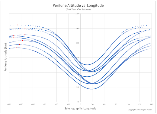
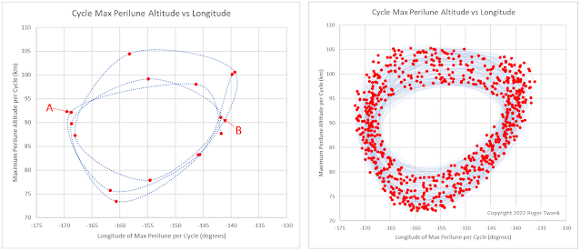
OK, we are able to focus the impact times, but what about the impact locations? As hoped, as the impacts begin to cluster more tightly around the desired time on May 29th, they also begin to cluster more tightly on the surface of the Moon. As I showed in a previous post, initially the impacts are spread across a wide band of longitudes, from 62° E to 126° E. That band is over 1000 miles wide! Figure 4 shows the results after nudging towards the target impact time. The impacts are now clustered around a few prominent terrain features near 10° N and 105° E. Although this is still quite a large area, we are making progress. The total search area is greatly reduced, especially since the impacts are concentrated primarily along crater rims. I'm beginning to have hope that Orion's final impact crater might be found. 

Figure 4: Locations for simulated impacts that occur near the time of the May 29th seismic event

Perhaps there are other clues we can use to further constrain the impact area...next time. Meanwhile, happy hunting!

Orion's Time of Impact

In a previous post we found that the Apollo 16 Lunar Module “Orion” probably hit the Moon in late May, 1972. It would be great if there was a database that could help us to pin down the time of impact more precisely, which would help to narrow the area of the impact. It turns out there is such a database, which is the seismic data collected from the Moon by the Apollo Passive Seismic Experiment, the PSE. The PSE probably recorded the impact of Orion, but in 1972 the impact would not have been recognized as that of a Lunar Module. With our modern simulations could we pick out a seismic event from all that data? Let’s check it out.

Figure 1: One of the PSE detectors, in the foreground, as deployed on the Moon. The Apollo 11 detector overheated after a few weeks, so the later ones were insulated with a reflective blanket.

Seismometers were placed on the lunar surface by each of the Apollo missions up to and including Apollo 16. The one from the Apollo 11 mission failed after two months, but in May of 1972 all of the other stations, from Apollo 12, 14, 15, and 16 were operating and their data was being continuously recorded back on Earth. (Lots of data, which consumed thousands of the open reel magnetic tapes used to record it at the time.) Over the next decade the data was analyzed, and a catalog of lunar seismic events was published in 1981. This catalog is available online today, in its coded format, along with an explanation of the coding. The analysis showed that the events had different characteristics, and could be grouped into various categories such as deep moonquakes, shallow moonquakes, and meteoroid impacts. 

One of the most unexpected features of the Moon became apparent as soon as the first seismic data began streaming back to Earth. To the surprise of the scientists, seismic events on the Moon lasted much longer than anticipated. Unlike Earth, where water and other viscous material dissipates seismic energy, the Moon is very brittle and completely dry, so there is much less absorption of the waves as they propagate around. One of the scientists went so far as to say that the Moon “rings like a bell”. Of course, this shouldn’t be taken literally…but moonquakes definitely reverberate much longer than earthquakes.

One interesting category of seismic event are those from the intentional impacts of Apollo hardware. There are 4 known events from discarded Lunar Modules, as shown in the table below. The table shows the date, the time when the seismic signals started and ended, and the peak amplitudes at each of the 4 PSE stations. The first is the Apollo 12 Lunar Module ascent stage, which crashed near that landing site in November, 1969 right after the placement of the A12 PSE station. Of course at that time the A12 station was the only one operating. For each subsequent LM impact, another station was operating. Also notice that the amplitudes tend to be largest at the newest station. That’s because the LM’s were usually crashed near the most recent landing site. This page lists the impact locations of these Lunar Modules, along with other impact locations. No PSE station was added for Apollo 17, so that impact was more distant from the stations. Notice that in all cases the vibrations lasted for more than one hour. The A12 impact lasted 65 minutes, even though it had a shallow impact angle. The A17 LM impact waves lasted over two hours.

Figure 2: PSE event data for the 4 known Lunar Module impacts

The impact of Orion would not have been recognized as an LM event in 1972. There was no tracking of the stage once its batteries died, and the modeling and computing at the time was insufficient to predict when Orion’s orbit would destabilize. Orion’s impact would have looked like a meteoroid event. Given that we see from simulations that Orion likely struck the Moon at the end of May, 1972, are there any meteoroid impact events in the catalog that could represent the demise of Orion?

Below is a list of all the catalogued meteoroid (type ‘C’) impact events between May 23rd and June 6th of 1972. Remember that in our first set of simulations, all the impacts occurred between May 28th and June 3rd. Notice that there is only one meteoroid event in that period, on May 29th. That is a very interesting event, given that it is right in the middle of the range of the trials. Could this be the impact of Orion? It lasts 98 minutes, and generates substantial amplitudes at all the stations. There is also a cryptic comment: “DIST”.

Figure 3: All the PSE meteoroid impact events from around the end of May, 1972. The May 29 event seems particularly interesting as a possible record of Orion's impact.

In searching the web for PSE data, one name comes up again and again: Dr. Yosio Nakamura. He was obviously deeply involved in analyzing all the data, as his name appears on many of the publications. Even the catalog of PSE events is tied to his name. As this article explains, he was intimately involved in the PSE project from beginning to end. He helped to capture and analyze the first data from Apollo 11, and was back in Houston for Apollo 12. He also helped to preserve the data in the 1990’s, by arranging for all the raw data of over 12,000 reels (!) of the original tapes to be transferred to more modern, and more compact Exabyte cassettes. Today he is an emeritus professor at the University of Texas in Austin.

I contacted Dr. Nakamura, explaining my interest in the meteroid event of May 29, 1972, and he was kind enough to reply back. Not only that, but he was also kind enough to visit the facility where the raw data is stored, examine the event records, and perform some analysis. Here is what he was able to say: 

“Two things are clear: (1) The recorded amplitude at the Apollo 16 station is definitely larger than that at the Apollo 14 station, even considering that the Apollo 14 station tends to record amplitude slightly larger than that at the Apollo 16 station because of local site effect.  This means that the impact location is east of the seismic network.  (2) Seismic signals are detected at all four stations.  This means that the impact location is not far into the far side of the moon, because if it were, the seismic signals would be significantly reduced because of the high shear-wave attenuation in the lower mantle.”

These facts do fit with the simulation results for Orion, which showed it impacting between 70 and 125 degrees East longitude. Was there any way from the timing of the signals to triangulate the impact location? 

“Because the onsets of the seismic signals of the {May 29} event are too weak to be read precisely to compute the impact location, I have been looking at the amplitudes of their signals instead. One of the attached files shows plots of the catalogued amplitudes vs. distance of the {May 29} event with suggested impact locations compared with those of the other LM impacts. In the top figure, the catalogued amplitudes are plotted, while in the bottom figure, catalogued amplitudes are adjusted, or compensated, for the difference in detection sensitivity among stations."

Below is Professor Nakamura's "bottom" figure, with the compensated amplitudes

Figure 4: Nakamura's plot of compensated PSE amplitudes versus distance for the known LM impacts, as well as for theoretical Orion impacts at two longitudes. This is the "bottom plot" that he refers to.

"One thing that is clear from the bottom plot is that there are some differences in the amount of seismic energy radiated from LM impacts:  Similar amount of energies were radiated from 14 LM and 15 LM impacts, while 12 LM impact radiated less energy, producing about 1/2 of the first two in seismic amplitudes and 17LM impact radiated more energy, producing about 3 times more amplitudes than the first two.  This happened even with nearly equal impact energies (3.14-3.43 x 10^9 J) and impact angles (3.2°-4.9° from horizontal) (NASA TM X-58131, Table 4-111)."

"Considering this range of observed amplitudes, the amplitudes and the distance ranges of the assumed impact location of the {May29} event are consistent with those for a LM impact.  If anything, it radiated more energy than the 14 and 15 LM impacts but similar to the 17 LM impact, and/or it may have been closer to the seismic network than assumed.  One thing we cannot do with this set of amplitude data is to pinpoint the impact location within say better than ~30° or `~1000 km or so in any direction.”

He then adds a final valuable clue…

“I estimate the time of this impact to be about 7 minutes before the cataloged time 21:22 UTC, or about 21:15 UTC, with an uncertainty of ±2 min. This is based on an impact distance of 3000±1000 km from the nearest station.”  [See the comment below.]

Wow! The simulations pointed us to one of the events in the PSE catalog. This event seems to fit well with what we know so far about Orion's orbit. The event is "consistent with those for a LM impact" at the range of impact locations we simulated, and if it's right, we now know fairly precisely the time of Orion's impact. With that information, we should be able to go back and refine the simulations, focusing on those that result in impacts at the stated time. That should GREATLY narrow down the area where Orion could have impacted. Could we actually locate the impact crater? 

I want to express my gratitude to Professor Nakamura for his kind assistance. I feel very fortunate to have benefitted from his expertise. Thank you!

More on Orion

Based on an initial simulation it seems that the Apollo 16 Lunar Module Orion, abandoned in lunar orbit in 1972, smashed into the surface of the Moon about 5 weeks later. Would it be possible to locate the impact crater? Let’s get the best estimate we can for the initial orbit, run a randomized series of simulations, to try to narrow the search.

In previous investigations I have relied on the Mission Reports to provide the initial orbit state. For Apollo 16, the record is much richer. In particular, there are orbital state vectors (i.e., position and velocity information) for each of the hundreds of photographs taken by the “Metric Camera” experiment, which was in the science bay of the Command Module. In particular, this file has all the state information for every photo taken during the mission. 

A subset of these is of special interest…those from the “Rev 60” and “Rev 63” mapping passes. This refers to the fact that the photos were all taken during the 60th or 63rd revolution of the Apollo 16 CSM around the Moon. By this time John Young and Charlie Duke had returned from the lunar surface, and rendezvous and docking took place during Rev 53.  The LM was jettisoned during Rev 62, so the Rev 60 and 63 mapping passes bracket the last known position of Orion.

I grabbed a set of the Rev 60 data points and adjusted a simulation so that I fit them as closely as I could. Though trial and error I found that I could match them to within +/- 20 meters of altitude. Based on the documentation, this original state vector data was fitted in 1972 to a solution for the orbit that was generated using the best gravity model and ephemeris available at that time. I’m using a better gravity model and a modern ephemeris, so I’m not surprised that I don’t match up exactly. A residual error of +/- 20 meters seems pretty good.

Then I did the same thing for Rev 63 data points to get another estimate of the CSM orbit after the LM was jettisoned. With these estimates for the orbit, I can propagate to the moment of jettison and compare to the values published in the Mission report. (The simulator can run “backwards”, so it can reverse propagate from Rev 63 just as easily as it propagates forward from Rev 60.) The results are shown in Figure 1.

Figure 1: Comparing Orion's initial state, from 3 different sources.

Not bad! The positions are all within 0.5 km of each other, and the velocities match up well. The velocity difference when working backwards from Rev 63 is slower than the others, which is expected…it accounts for the ~2 ft/sec separation maneuver performed after Orion was jettisoned. 

The next step is to compensate the horizontal flight path angle, i.e., the HFPA. Orion was jettisoned “upwards”, away from the Moon, at about 2 f.p.s. and so this slightly increases the angle that it is moving relative to the local horizontal direction. It works out to be about 0.021 degrees, so adding this to the HFPA gives 0.42 degrees.

Now we can generate random sets of initial conditions that are similar to these and see where the impacts occur. I adopted the "Rev 60" state as the “nominal” case, and then varied randomly around those values. I generated a total of 350 randomized parameter sets and ran them all. Each run takes about 8 minutes to simulate, and I have a python script that automatically runs then one after another, so the whole batch completes in about 2 days. Each run produces a ground track file, and I post-process all of these as a batch to extract the impact locations.

What are the results? All 350 simulated impacts occurred between May 28th, and June 2nd of 1972. That's a fairly tight cluster. Looking deeper, there are some things that were expected, and other things I found surprising. Figure 2 is a plot of the impact date versus impact longitude for all 350 trials. The first thing to notice is the overall trend. Impacts that occur earlier are farther to the East, and the later ones are progressively farther West. This is to be expected, because the Moon is rotating Westward under the orbit as it destabilizes. (The impacts are also focused in a narrow band of latitudes, from 8.5 to 10 °N, which is under the plane of the orbit.)

Figure 2: Impact Longitude versus Date. Later impacts occur farther West.

Then notice the next trend…the impact longitudes occur in bands. For instance, notice that near the end of May 29th, the impacts are mostly around 104 °E, and then during May 30th they shift and are clustered around 99 °E. This clustering also isn’t surprising…it’s a consequence of the lunar terrain. The impacts always occur on the highest nearby terrain as the orbit drops lower and lower, so these impact clusters correspond to tall features of the Moon’s surface. Figure 3 below shows the latitude and longitude of the impacts (as red dots) superimposed on a map of the Moon, and it’s obvious that the dots are clustered around craters and mountainous areas. (At this scale it's hard to see that there are a lot of overlapping dots.)

Figure 3: Impact locations superimposed on a map of the Moon.

One thing I did find surprising is that the impact times are also quantized…they tend to be concentrated into buckets separated by about two hours. A lot of the individual impacts are overlapping on the plot in Figure 1 above, so it’s easier to see this time quantization if we zoom in on a few impacts like in Figure 4 below. Now you can see that there are 6 trials that resulted in impacts around 20:00 hours (10 PM) on May 29th, then 3 others around 22:00, then another 4 around Midnight, and so forth. On the one hand, the two-hour separation makes sense. If the spacecraft barely misses a mountain on one pass, it is likely to be lower, and therefore to impact that mountain on the next pass, which will come two hours later. (The time to complete one revolution is about two hours.) But all the trials have slightly different orbits and slightly different periods, so after 5 weeks orbiting the Moon all those virtual spacecraft in all those trials should have spread out, like race cars around an oval track in a long race.  

Figure 4: Details of impacts occurring around midnight on May 29th, showing how the impacts are occurring in clusters separated by about 2 hours.

It turns out that they do spread out, but the ones that are in similar orbits, with similar orbital periods, tend to impact around the same time. So, the impact times are sorted by orbital period. I would not have guessed this, but in hindsight it also makes sense. It turns out that the impact times depend on the energy of the initial orbit. Lower energy results in earlier impact, and vice versa. The energy of the orbit also determines the orbital period. Therefore, impacts that occur around the same time, which started with similar energy, also have the same period, resulting in the clustering of the impact times. Figure 5 below shows a plot of initial orbit altitude versus impact time, and there is a clear relationship. (The altitude plotted is the average of the initial apolune and perilune altitudes, which directly ties to the orbital energy.)

Figure 5: The time of impact correlates to the initial energy of the orbit, which also relates to the orbital period. This explains the clustering of the impact times.

What have we learned so far about Orion? It seems clear that Orion must have impacted the Moon sometime around the end of May of 1972, about 5 weeks after it was jettisoned. Longitude of the impact is probably between 70 and 120 °E. The impact location is likely to be on a mountain or crater wall, along a narrow track between 8 and 11 °N Latitude, and there seem to be just a handful of locations where the impacts are concentrated. Could we actually locate the impact crater? Although we have narrowed down the search considerably, we are still talking about huge areas of the Moon. (One degree of longitude along the Moon's equator is about 20 miles.) In my next post we'll dig into some other sources of data to see if there are any clues that could be helpful to narrow the search even more.

What About Orion?

As I write this, the 50th anniversary of the Apollo 16 mission is a few months away. Like all of the later Apollo missions, the plan for the ascent stage of the Lunar Module “Orion”, after it returned the astronauts to orbit, was to intentionally crash it into the lunar surface. This would generate seismic waves that would reveal the inner structure of the Moon by way of the seismometers left on the surface by the astronauts. These intentional impacts were done for the Apollo 12, 14, 15, and 17 missions. But something went wrong during Apollo 16, and the LM “Orion” stage did not hold its attitude (orientation) after it was jettisoned. With no way to control which way it was pointing, there was no safe way to command its engine to fire. It was abandoned in orbit, left to drift under the forces of lunar gravity, and no one knows what happened to it. Let’s turn our attention to Orion and see if we can shed some light on what became of this vessel.

If you’ve read my previous posts, you know the drill by now. We can get the initial conditions for the stage orbit from the Mission Report. We use GMAT and a high-fidelity gravity map to simulate the spacecraft. We record the “perilune”, the lowest point, for each revolution, and watch to see how close the stage comes to the surface over time. The orbital period is about two hours, as usual for low lunar orbits, so we get about 12 perilune points per day. GMAT simulates one year of spacecraft time in about an hour (on my computer) so we get a month of simulated orbit data every 5 minutes or so. The simulator doesn’t know about terrain, but we can tell the simulator to stop once the perilune point is a few km below the mean radius…at a point where an impact would surely already have occurred.

Figure 1: Simulated Perilune Altitude for Orion

Using the “nominal” initial conditions from the Mission Report, I get a script like this one. And the resulting perilune sequence is shown in Figure 1. It looks like Orion didn’t remain in orbit very long. By the end of May 1972, the spacecraft is already zero km above the Moon’s mean radius. A day or two later the perilune has dropped to 5 km below mean radius. Whack!

If you read my earlier post about “PFS-2” the Apollo 16 subsatellite, you might notice something interesting. The perilune sequence looks very similar, and PFS-2 is known to have also impacted the Moon near the end of May. Did I use the wrong script? No, actually the similar result is not surprising, when you consider the release of each object. Figure 2 shows an excerpt from the Mission Report, and details the sequence. After Orion was jettisoned, the astronauts performed a small “separation burn”, changing their velocity by just 2 feet per second. Then an hour later they released PFS-2. So, Orion was drifting along nearby when PFS-2 was jettisoned, and the two objects were in very similar orbits. They were in almost the same plane, and at almost the same altitude and speed. In hindsight it is not surprising that both orbits destabilize in a similar fashion.

Figure2: This excerpt from the Mission Report shows how the PFS-2 subsatellite was launched soon after Orion was jettisoned. Both events are during the 62nd revolution around the Moon, and just one small "CSM separation" maneuver was performed in between. Thus Orion and PFS-2 were in very similar orbits. Similar impact dates should not be surprising.

Where does Orion impact the Moon in this nominal case? Using the analysis method I describe here, Orion strikes the Moon at 77.5E, 8.16N at 8:14 on June 1st, 1972. Again, that is very similar to the impact time and point reported by NASA for PFS-2. The time is day or so later, and the impact is farther West. This simulation runs fairly quickly, completing in under 10 minutes on my computer. That means it will be quick to run a lot of variations of the initial conditions, so as to understand how much uncertainty there is in the result. I'll post those results later.

There is another important source of data we can look to for clues about Orion: those seismometers left on the surface that I mentioned above. In May of 1972 NASA had 4 stations operating, at the landing sites of Apollo 12, 14, 15, and 16. (The station at the Apollo 11 site stopped working late in August of 1969.) The data from all 4 stations was monitored and recorded continuously. The impact of Orion, weighing 5,000 pounds and moving at a mile per second, should have registered as a meteoroid strike, so we’ll be able to look for seismic events that might help to pinpoint the time of impact.

And then, in addition to the Mission Report, there are other clues we can use to help understand Orion’s initial orbit. During the later Apollo Missions, including Apollo 16, an extensive set of photographs were taken from lunar orbit by Panoramic and Mapping Cameras operating in the science bay of the Service Module. Each of these photos has an associated blob of data about the location of the spacecraft when it was taken. Hopefully this data can be used to further refine the initial conditions. And then if we get very lucky, these photographs might contain a “before” view of the area where Orion hit the surface, making it easier to identify any “new” crater.

Okay, so we have a large spacecraft that struck the Moon within weeks of its last sighting. We have a number of great data sources that we can search for clues. We have photos of the surface taken before the impact, and of course we have the high-resolution images captured by LRO and other lunar satellites. Perhaps we can identify the impact crater of Orion in time for the 50th anniversary of the mission. The game is on!

Impact Analysis

 

The simulation environment I am using, GMAT, doesn’t know anything about the Moon’s mountains or valleys. When it calculates the altitude of an orbit, that altitude is relative to the “mean radius” of the Moon, somewhat comparable to “sea level” on Earth. So far, in the simulations I have run for the Eagle and Snoopy, that hasn’t mattered, because the orbits of both objects remain high above the surface. But to estimate the location of a possible impact, as for the Apollo 16 subsatellite, we have to do a deeper analysis. In this post I’ll explain how that works. 

Let's start with the big picture. An orbit has become more eccentric…the high point of the orbit has moved higher, and the low point of the orbit has moved lower. On Earth, as the spacecraft began to skim the atmosphere, it would slow down, then burn up, and the heaviest bits might make it all the way to the surface. Since the Moon has no atmosphere, the spacecraft, at the low point of its orbit, can zip past the lunar surface at very low altitude, moving more than a mile per second, and if it misses the surface, even barely, it can continue around for another pass. 

Figure 1: The path of a spacecraft passing low over the Moon's surface

If the Moon were a smooth ball the impact might occur at the lowest approach. However, the Moon is not so smooth. In fact, it is quite rough, with jagged surface features thrown up by countless meteoroid impacts, undiminished by wind or rain. If a spacecraft comes streaking by and strikes the surface, that impact will likely be on a piece of high terrain, perhaps the side of a mountain or a crater wall. To work out the location, we’ll need a good elevation model of the Moon’s terrain. Fortunately, these are freely available, with resolution as high as 512 points per degree, which works out to one elevation point for every 100 feet or so.

We also need the simulator to give us a full “ground track” record, instead of just the lowest point of each orbit. The ground track is a list of latitude, longitude, and altitude points and typically a point is recorded for every 10-20 seconds of simulated time, as in the example shown below. Given that the spacecraft is traveling at about one mile per second, there is a lot of ground between each point. It’s not enough detail to locate the impact exactly, but it shows us the places where the spacecraft is close to the surface…places where we can zoom in for a closer look. As we go through this exercise, we will be zooming in on the points highlighted in green.

Figure 2: Ground track file excerpt. The terrain and "AGL" altitude data (in km) was added by post-processing the output from the simulator.

The first thing we need to do is to “post-process” the ground track file, looking up the height of the surface for each point in the file. For this method I am greatly indebted to a space enthusiast named Daniel Estevez, who ran simulations to try to estimate the impact location of a lunar satellite and posted his results here. I use a modified version of his method, wherein I run two passes on the ground track file.

Step one is to go through the ground track, one line at a time. From the latitude and longitude, we can look up the nearest terrain altitude point in the elevation model. Once we know the spacecraft altitude and the terrain height, we can calculate its “Above Ground Level” altitude. I write out a new copy of the ground track file with the extra terrain altitude and “AGL” data points added to each line, like the yellow values shown in the figure above. To limit the size of the new file I discard any point where the spacecraft is more than 5 km above the surface.

Here is a plot of a ground track file showing two low revolutions of a spacecraft over an area of the Moon. One thing to notice right away, even though this is covering 30 degrees of longitude, or a distance of about 900 km, the "zero" altitude point is flat, and the satellite trajectory curves upward, away from the Moon. This is just to make it easier to plot out the data. I promise the Moon is NOT flat, and the spacecraft is always curving towards the center of the Moon, as in Figure 1 above. The flattening of the Moon for this chart doesn't affect our ability to find the impact point. Another thing to keep in mind is that the vertical scale is greatly exaggerated. This chart is 900 km wide and just 8 km high.

Figure 3: A "flattened" plot of low passes of a spacecraft over the Moon. The area in the green box depicts the values highlighted in green from Figure 2.

Figure 3 allows us to see the areas where the spacecraft is coming close to the surface of the Moon. In particular, the points in the small green box highlight the closest approach visible at this resolution, and the closest point shows a separation of 449 meters above the ground. Given that these two data points are separated by a distance of over 20 km, we need to zoom in and take a closer look.

Figure 4: A "zoomed in" look at the region of the green box from Figure 3. We see that the spacecraft altitude is lower than the terrain altitude at 98.97°. Kaboom!

The figure above shows the zoomed in view. The two red dots are the points from the green box of Figure 3, the same data points highlighted in the ground track file in Figure 2.  What we have done is to make a straight line between these points, and break that line into 100 shorter segments, like the dotted blue line. (This process is called linear interpolation.) For each blue dot we can again look up the terrain altitude and compare it to the spacecraft altitude. Sure enough, in that intervening 20 km between the two red points there was a mountain, about 800 meters tall, and the spacecraft (moving from right to left in this example) strikes it near its top, at around 98.97°. 

How do we know there wasn't another mountain lurking somewhere further to the East? We don't! We have to check. In my code, posted here, I check any time I find a point that is within 3 km of the ground. (I also tried higher thresholds, but 3 km seems to be sufficient to catch all the lurking mountains in my tests so far.)

This is how I have used GMAT to estimate the impact location of the Apollo 16 Particles and Fields Subsatellite, the notorious (in some circles) PFS-2. Now that I have this tool working, I am interested to use it to investigate another Apollo impact. Yes, there is another spacecraft from the Apollo era whose final resting place is unknown...the ascent stage of the Apollo 16 Lunar Module "Orion". As I write these words the 50th anniversary of that mission is fast approaching. Stand by for further updates.

A Reality Check

 What about that Apollo 16 subsatellite?

In this blog I have shown that two Apollo spacecraft were left in orbits that are stable over decades. That’s really surprising and unexpected. Some people have asked if I can simulate an object that is known to have decayed out of orbit, as a reality check, to show that these simulations aren’t out of whack. That’s what we’ll do in this post.

One very notable case is the Apollo 16 Particles and Fields Subsatellite, otherwise known as PFS-2, which decayed out of lunar orbit in 1972 after only 5 weeks in orbit. Weighing just 36 kg, it was jettisoned from the Apollo 16 Service Module not long before the crew left lunar orbit to return to Earth. Originally it was planned to raise the orbit of Apollo 16, so that PFS-2 would remain in orbit for a year. Due to problems during the mission, that orbit change was skipped, and the expected orbital lifetime of PFS-2 was cut down to a few months. PFS-2 was equipped with a transmitter so that it could be tracked, and its data could be sent back to Earth. Only 34 days after it was jettisoned, the transmissions ceased, and PFS-2 impacted the Moon. 

Let’s run a simulation of PFS-2 and see what happens. As with previous simulations we can get the initial conditions from the Mission Report. The Figure 1 shows the data from the report. I believe the report is showing the state of the Command-Service Module (CSM) rather than the PFS-2, but it should be close enough to see if we are in the right ballpark. After converting the parameters to metric and getting them into the right coordinate frame, I get a GMAT script like this one, posted on GitHub.

Figure 1: Showing the initial conditions of PFS-2 from the Mission Report.

For starters, we’ll just record the low point in each revolution, as we have done previously. Figure 2 shows how it looks over time. We see the minimum altitude dropping for several weeks, and then there is a reversal and it starts to rise up again around the middle of May. About a week later the orbit starts to become more eccentric, and the perilune altitude begins dropping again. Sure enough, just 5 weeks after jettison, at the end of May 1972, the low point of the orbit is below the average radius of the Moon...zero altitude...and that is a sure sign that impact has occurred. (The simulator doesn’t check for impact while it is running…it will happily simulate an object that is actually beneath the surface, so we’ll have to look in greater detail to see exactly when and where the impact occurs. I’ll explain how to do that in a future blog post.)

Figure 2: Simulated perilune altitude.

A more detailed analysis of the simulation results gives the location and time of impact, and it comes out as below. Tracking data from the satellite ended shortly after 10:31 PM on May 29th, with an estimated impact at 111° East longitude, and 10° North latitude. This simulation puts the impact about 14 hours later, and about 13 degrees further west. That's not bad! 

Figure 3: Impact times and locations reported by NASA and estimated by simulation

There is another source of information on the PFS-2 initial orbit, at this page. It describes the orbit in a different way, and the parameters don’t completely agree with those in the Mission Report. If we run again with those initial conditions, we get the results labelled “Nominal 2”. This time we get closer to the 1972 estimated impact location and time…impacting about three hours earlier and about 4° more to the west, with the latitude agreeing almost exactly.

In my view, the basic answer is “yes”, these simulations do compare well against reality. We are able to predict the impact of PFS-2 within a few hours of the actual time, and within a few degrees of the estimated location. Considering the uncertainty of the initial conditions, with two different NASA sources that don’t agree, errors of a few hours either way don’t seem too surprising. Having gone through this exercise, I have even greater confidence in the results obtained for Eagle and Snoopy.

By the way, if you are looking for a lunar sleuthing challenge, the actual impact crater of PFS-2 has never been located. This web page states that the original raw PFS-2 tracking data has been preserved, and if you were to obtain that data and fit a simulation to it, I suspect you would be able to map out a very small area where the PFS-2 impact occurred on the surface of the Moon almost 50 years ago. You might be the person to identify the final resting place of the infamous short-lived Apollo subsatellite. Good luck and happy hunting!

Feedback and Stability

The Moon’s uneven gravity field causes most lunar orbits to be unstable. Over time the orbits increase in eccentricity, which is to say that the high part of the orbit gets higher, and the low part gets lower, until the object strikes the lunar surface. In this blog I have described the orbits of two different Apollo artifacts that show long-term stability in their orbits. (The Eagle and Snoopy.) They somehow manage to evade the instability that dooms most lunar satellites. How could that be? In this post we’ll dig in deeper to try to understand what is going on in greater detail.

I’ll start by focusing on the Eagle, and then at the end we can do a similar analysis for Snoopy. To start, as a reminder, look at the way the perilune altitude varies over time in the figure below. (Remember, perilune altitude is the lowest point of each revolution.) You see a cycle that repeats as the minimum altitude dips lower then climbs higher about every 25 days. I showed in a previous post that this 25-day cycle reflects the way the orbit changes as the Moon rotates underneath. The lowest lows always occur on the near side of the Moon. The fact that the cycle completes in 25 days, while the Moon completes a full rotation in 27.32 days, means that the Eagles orbit is also precessing. (This is also sometimes called “Apsidal advance”.) In this way the long axis of the Eagle’s orbit, called the Apse Line, does a complete circuit of the Moon in about 25 days, and this drives the short-period variation.

Figure 1: Minimum altitude of the Eagle in the first year after jettison. Notice the shorter variations every 25 days, and the longer variation every 4-5 months.

What about that longer variation in the perilune altitude? Notice how every 4-5 months the minimum altitude goes higher and then lower. What’s going on there? If you look at the figure above, notice that the minimum altitude is nearly the same at point A and point B, but somehow this system “knows” that at point A the longer cycle is increasing, and at point B the longer cycle is decreasing. Somehow there is “state” information being stored in the system, so that it “remembers” where it is in the long-period cycle. Let’s dig in and look for that “state” signal.

Figure 2: Showing the time (in days) between the peaks of the first 4 complete cycles for the Eagle. Notice that the time between peaks increases as the altitudes move lower.

For starters, let's look for differences between the “low” cycles and “high” cycles. One thing to measure is the “period” of the cycle, i.e., how many days it takes to complete a cycle. We can measure the time between the highest point in each cycle. In figure 2 above, I show the time (in days) to go from one peak to the next for the first 4 complete cycles of the Eagle’s orbit back in 1969. Do you notice anything interesting? As the altitudes get higher, the times get a bit shorter. As the altitudes get lower, the times get a bit longer. We can plot these on a graph that makes the relationship easier to see, and in the figure below I show the first 14 cycles…the first year of the Eagle after jettison. If I plotted out the data for 52 years you would see that the same relationship continues to the present day. This is a persistent feature of the Eagle's orbit.

Figure 3: Cycle length and end peak altitude for 14 Eagle cycles during its first year in lunar orbit.

The next thing to notice about these cycles is how they relate to the Moon. The plot below shows perilune altitude versus the Moon’s longitude, for one year. As the Moon rotates underneath the orbit, we see 14 tracks wrapping around. Each of the blue dots represents the lowest point of one revolution, and the longitude where that low point occurs above the Moon. What’s interesting is that the lowest parts of the cycles always occur on the near side of the Moon, near 30 degrees East, while the highest parts occur on the lunar far side. (From Earth we can only see lunar longitudes between -98° and +98°.)

Figure 4: Mapping how perilune altitude varies with lunar longitude. Eccentricity of the orbit is highest when perilune occurs on the near side of the Moon.

You might also notice some “sloshing” back and forth in that pattern in Figure 4. Notice on the left part of the figure where the highest points in each cycle are marked with red dots. The dots actually form a loop. It's even more interesting to connect the successive dots, as in Figure 5 below. In this figure I’m only showing the highest points of each cycle, like the red dots above, but now I added a dotted blue line showing the sequence. You can see that over the course of a year these dots trace out a series of loops. And these loops tie back to the slower 4- to 5-month variation you see that first figure above. Now we can see the difference between points A and B in the first figure. I’ve marked them again in Figure 5. Point A occurs about 30 degrees farther to the East than point B. This longitudinal variation is how the system stores its “state” information…how it “remembers” whether the short cycles are increasing or decreasing. And just to be clear, this is another pattern that is stable over decades. On the left in Figure 5, notice how this variation looks over a 50-year period. It doesn’t expand or contract or drift away. It remains centered on this longitude.

Figure 5: These plots show the lunar longitude where the perilune cycle peaks occur. Points A and B on the left are the same ones marked in Figure 1. All the red points on the left are also marked in red in Figure 4. Data for 50 years is plotted on the right, showing the long-term stability of the pattern.

We’ve seen how the eccentricity variation of the orbit stays locked to lunar longitude over decades. How can that be? There must be some feedback mechanism that prevents it from drifting away. It’s interesting to look at the rate that the perilune longitude point changes. To do that, for every revolution, we have to measure how far Eastward the perilune point shifted and compare that to the elapsed time. If we divide the longitude change by the elapsed time, we get a measure of the rate. (The elapsed time is nearly constant…about 1 hour and 58 minutes per revolution, but it’s a spreadsheet doing the math, so why not recalculate it for each point.) I’ll call this measurement the “precession rate”. That’s kind of a misnomer…the longitude is mostly changing because of the Moon’s rotation under the orbit, which is not really precession. (This component is also constant, because the rate of the Moons rotation is constant.) But there is an additional precession in the orbit so there is some variation in this precession rate. Here it is...

Figure 6: The "Precession Rate" varies depending on perilune altitude.

What is interesting here is that the rate gets much faster as the perilune altitude gets higher. Put another way, the precession rate varies inversely with eccentricity. As the orbit becomes more eccentric, the rate slows down. As the rate slows down, the Moon's gravity begins to drive the eccentricity lower. Lower eccentricity causes the rate to speed up, and the cycle repeats. Again, and again. For decades.

OK we found an interesting pattern in the orbit of the Eagle that persists for decades and can plausibly explain its long-term stability. (“Explain” is a strong word here…I believe there are more layers to this onion.) How about the Snoopy descent stage? If we go through the same exercise with Snoopy, we see very similar patterns. Compare the figures below for Snoopy’s orbit to those above for the Eagle. There is something about these retrograde equatorial orbits that leads to long-term stability, somehow evading the unstable fate of most other lunar satellites. Pretty cool, eh?

Figure 7: These plots of Snoopy's orbit data show similar patterns to those of the Eagle. A similar feedback mechanism seems to be responsible for the long-term stability displayed by both orbits.